MATLAB program for Ground response analysis or FreeField acceleration response of Gilroy soil site

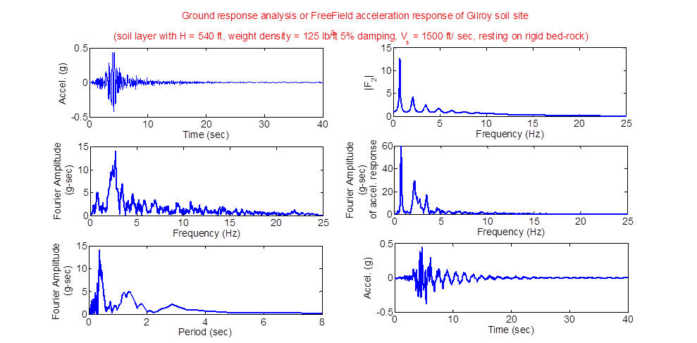
Ground response analysis or FreeField acceleration response of Gilroy soil site

(soil layer with H = 540 ft, weight density = 125 lb/ft^3, 5% damping, V_s = 1500 ft/ sec, resting on rigid bed-rock)

Ref: Kramer 1996, Example 7.2 in page 262

Fig. 1. Soil layer resting on rigid bed-rock

Gilroy Ground motion (Gilroy# 1, Rock) - Acceleration time history data

https://strongmotioncenter.org/vdc/scripts/stnpage.plx?stations=563

Steps in the MATLAB program for free-field analysis

1.      The acceleration time history given in the above table is saved as MATLAB data file Gilroy1_ATH.mat. This is the acceleration at the bed-rock below the soil laer.

2.      It is padded with zeros for end-correction in DFT

3.      Fft() function is used to split the time history into harmonics

4.      Also, the transfer function (F2) is generated for each frequency

5.      Product of fft() and transfer function gives the frequency response of acceleration at the top of the soil site

6.      To get the time response of acceleration at the top of the soil, ifft() function is used

MATLAB Program

% Importing the ground motion time history clear;clc; load ('Gilroy1_ATH.mat');dt=0.02;H=540;ro=125/32.2;G=(ro)*1500^2;zi=0.05; N=length(data);N=2^(ceil(log2(N)));data=[data;zeros(N-length(data),1)]; t=dt*(1:N)';freq=(1:N)'/dt/N; figure;subplot(3,2,1);plot(t,data); FAmp=fft(data);absFAmp=abs(FAmp(1:N/2)); subplot(3,2,3);plot(freq(1:N/2),absFAmp); subplot(3,2,5);plot(1./freq( 1:N/2),absFAmp); w=2*pi*freq;vs_=sqrt(G*(1+2*1i*zi)/ro); F2=1./cos(w*H/vs_);absF2=abs(F2); subplot(3,2,2);plot(freq(1:N/2),absF2(1:N/2)); Afw=F2.*FAmp;%Afw=abs(F2).*abs(FAmp);% subplot(3,2,4);plot(freq(1:N/2),abs(Afw(1:N/2))); Aft=ifft(Afw); subplot(3,2,6);plot(t,Aft);

Results

Deflection to BMD

Introduction: In many problems of structural mechanics, the deflection curve of a beam is obtained.
The displacement- based finite element method is one such process that gives deflections/ displacements/
deformations as the first level output, displacement being the field variable. Further quantities of interest
needs to be derived from this basic solution.   Here, I present a working procedure using MATLAB code
for generating the BMD and SFD from deflection curve following the assumptions of pure bending under
small deformations.

Algorithm:

Step1: Fit a polynomial of degree ‘n’ for the deflection data

Step2: Obtain the first derivative of the polynomial fit

Step3: Obtain the second derivative of the polynomial fit. This gives curvature

Step4: Multiply the curvature with flexural rigidity ‘EI’ of the beam to get BMD

MATLAB Code:

 

function [slope,curvature,BMD]=Deflection2BMD(x,y,EI,Order)    f=fittype(['poly' num2str(Order)]);%f = fittype('cubicinterp');    fit1 = fit(x,y,f);    [d1,d2] = differentiate(fit1,x);    subplot(3,2,1);    plot(fit1,x,y);ylabel('Deflection, y');% cfit plot method    subplot(3,2,3);    area(x,d1,'Facecolor','m'); ylabel('Rotation, dy/dx');% double plot method    grid on    legend('1st derivative')    subplot(3,2,5);    area(x,d2,'Facecolor','y');ylabel('Curvature, d^2y/dx^2'); % double plot method    grid on    legend('2nd derivative')    slope=d1;curvature=d2;BMD=d2*EI; end

Illustration:

Let us consider a cantilever steel beam of cross-sectional dimensions 250 mm x 300 mm (Very heavy ofcourse !!!)
 modelled by 3D soild/ brick/ hexhedral elements using Finite Element Analysis, under gravity loading.
The beam is 4 m long.   After completing the static stress analysis of the model under self-weight (gravity),
we can easily obtain the deflection curve of the axis of the beam. This is used as the input for the above
MATLAB function. The following is the result of the analysis.

By multiplying the last figure with EI, w get the BMD. It can be seen that the bending moment at the fixed end
is 481 kN-m (taking E=2E11 Pa). This is almost equal to the actual bending moment of a 4 m long cantilever
beam with a UDL of 6000 N/m (which is the self-weight of the beam taking 8000 kg/m3 as the density of steel).

MATLAB coding for generation of various yield/ failure surfaces used in Soil-plasticity

MATLAB coding for generation of various yield/ failure surfaces used in Soil-plasticity

Introduction: In this blog we will give (i) formulation of yield criteria in some plasticity models (ii) a MATLAB code that uses the formulation to generate the 3D yield surface in principal stress-space (iii) the MATLAB generated figures for some selected values of the parameters involved in the respective models.
Formulation: The yield/ failure criteria are expressed in terms of stress invariants ( I₁, I₂, I₃ )or deviatoric stress invariants ( J₁, J₂, J₃) or combinations of them. The plotting is to be done in principal stress space (σ₁- σ₂-σ₃). For the plotting of yield surface, the Haigh- westergaard coordinates (ξ, ρ, θ) are best means.Therefore, these principal stresses are to be expressed in terms of Haigh- westergaard coordinates (ξ, ρ, θ) using the transformation shown below




For Matsuoka-Nakai model, we need to do some extra formulations to obtain the yield surface in terms of I₁, J₂ and J₃, as follows,


Using this J₂ can be determined and on applying Haigh-Westergaard transformation, we get coordinates in principal stress space.

Original Cam Clay Model

 

Modified Cam-Clay model

Algorithm : For generating 3D yield surfaces, the following steps depict the sequence of implementation of plotting 

1. Taking the input parameters
2. Discretizing the axial coordinate [hydrostatic (p) pressures] and Lode Angles (th) , and forming grid of these values in Haigh-westergaard space
3. For each set of (p,th) values, the value of the radial coordinate (r ) is calculated based on yield criteria. This step will be different for each yield criteria
4. Applying the Haigh-westergaard transformation to get the coordinates in principal stress space (σ₁, σ₂, σ₃).

MATLAB code for these steps is shown in tables below, for Tresca, Matsuako-Nakai, Drucker- Prager and HiSS yielding criteria.


The plots resulting from execution of above MATLAB codes are shown below.