Structurallearnings

Tuesday, 14 April 2020

ILD for trusses in which panel points are not vertically in line with loaded panel points

In the following video, I tried to explain the procedure for drawing ILDs for member forces in trusses in which the top and bottom panel points are not vertically in line. In such trusses, a small correction needs to be done in the ILD. There should not be an abrupt change in the ILD at the point or section where the loading does not appear directly. So, that abrupt change at non-loading panel points needs to be smoothened.

Saturday, 11 April 2020

ILD s for Simply supported Bridge Trusses

The following video is for the students of II year B. Tech (civil Engineering) Programme. The video details the procedure for drawing ILDs of simply supported trusses

Wednesday, 8 April 2020

Unit Load method for deflections of rigid frames

The following video is for II year under graduate students of Civil Engineering Programme

Strain energy method for slopes and Deflection of beams

The following video is made for students of II year of Bachelor's programme in Civil Engineering

Friday, 15 February 2019

PLotting truss structures using MATLAB code

Objective: The following article explains the MATLAB code to plot a figure of truss structure to scale

MATLAB Functions used: line( ), min( ), max( ), length( ), viscircles( ), patch( ), etc

Other features: THe supports and loading are also depicted in the plots. The load values and directions are clearly indicated in color

MATLAB Code:

function drawtruss2D(NODE,ELEM,L_BC)
figure;line([NODE(ELEM(:,1),1) NODE(ELEM(:,2),1)]',[NODE(ELEM(:,1),2) ...
NODE(ELEM(:,2),2)]','Color','b','LineWidth',2,'Marker','o',...
'MArkerSize',8,'MarkerFacecolor','w');hold on;
minX=min(NODE(:,1));maxX=max(NODE(:,1));minY=min(NODE(:,2));maxY=max(NODE(:,2));
rangeX=maxX-minX;rangeY=maxY-minY;
xlim([minX-0.2*rangeX maxX+0.2*rangeX]);ylim([minY-0.2*rangeY maxY+0.2*rangeY]);
axis equal
if nargin==3
nl=rangeX*0.10;nb=rangeY*0.05;
for o=1:length(L_BC)
OType= L_BC{o}{1};
switch OType
case 'F'
X=[0;-nl*0.30;-nl*0.20;-nl;-nl;-nl*0.20;-nl*0.30;0];
Y=[0;nb;nb*0.2;nb*0.2;-nb*0.2;-nb*0.2;-nb;0]*0.7;
if length(L_BC{o})>4;X=X+nl;end
F=L_BC{o}{2};rot=L_BC{o}{3};
theta=rot/180*pi;
R = [cos(theta) -sin(theta); sin(theta) cos(theta)];
Trans=[X Y]*R;Xt=Trans(:,1);Yt=Trans(:,2);
Xf=NODE(F,1);Yf=NODE(F,2);
patch(Xt+Xf,Yt+Yf,[1 0 0]);
Xa=[nl*0.25 nb*0.25]*R;
if length(L_BC{o})>4;text(Xt(1)+Xf+Xa(1),Yt(1)+Yf+Xa(2),L_BC{o}{4},'FontSize',18);
else text(Xt(4)+Xf+Xa(1),Yt(4)+Yf+Xa(2),L_BC{o}{4},'FontSize',18);end
case 'H'
X=[0;-nl/4;-nl/2;-nl/2;nl/2;nl/2;nl/4;0];
Y=[0;-nb*0.8;-nb*0.8;-nb;-nb;-nb*0.8;-nb*0.8;0]*1.2;
F=L_BC{o}{2};rot=L_BC{o}{3};
theta=rot/180*pi;
R = [cos(theta) -sin(theta); sin(theta) cos(theta)];
Trans=[X Y]*R;Xt=Trans(:,1);Yt=Trans(:,2);
Xf=NODE(F,1);Yf=NODE(F,2);
patch(Xt+Xf,Yt+Yf,[0.5 1 0.5]);
case 'R'
X=[-nl/2;-nl/2;nl/2;nl/2];
Y=[-nb*0.4;-nb;-nb;-nb*0.4]*1.2;
F=L_BC{o}{2};rot=L_BC{o}{3};
theta=rot/180*pi;
R = [cos(theta) -sin(theta); sin(theta) cos(theta)];
Trans=[X Y]*R;Xt=Trans(:,1);Yt=Trans(:,2);
Xf=NODE(F,1);Yf=NODE(F,2);
patch(Xt+Xf,Yt+Yf,[1 1 0.5]);
viscircles([0 0]*R+[Xf Yf],nb*0.4,'LineWidth',5,'EdgeColor','y');
viscircles([0 0]*R+[Xf Yf],nb*0.6,'EdgeColor','k');
end

end
end
return

Typical input Files:

%Truss data for various problems
FlagNo=12;
switch FlagNo
case 1 % Single Braced Truss %Page 693 Vazirani and Ratwani
NODET=[0 0;8 0];NODE=[];for i=1:5;NODE=[NODE;NODET+[[0;0] 6*[i-1;i-1]]];end
ELEMT=[1 3;1 4; 3 4 ;2 4];ELEM=[];for i=1:4;ELEM=[ELEM;ELEMT+(i-1)*2];end
drawtruss2D(NODE,ELEM,{{'F',3,0,'30 kN',1},{'F',4,180,'30 kN'},{'R',2,0,'30 kN'},{'H',1,0,'30 kN'}});
case 2 %
NODET=[3 0;3 4;6 0;6 8];NODE=[0 0;0 8];n=4;
for i=1:n
NODE=[NODE;NODET+[6*(i-1)*ones(4,1) zeros(4,1)]];
end
ELEMT=[1 3;1 4; 2 4;3 5;4 5;2 6;5 6];ELEM=[1 2];
ELEMT1=[1 3;1 4; 3 5;4 5;4 6;2 6;5 6];
for i=1:n
if i<=n/2
ELEM=[ELEM;ELEMT+4*(i-1)];
else
ELEM=[ELEM;ELEMT1+4*(i-1)];
end
end
drawtruss2D(NODE,ELEM);
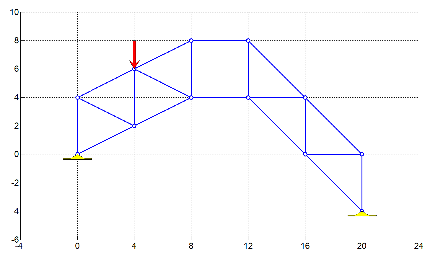
case 3 %Page 11 Vazirani
NODE=[0 0;0 4;4 2;4 6;8 4;8 8;12 4;12 8;16 0;16 4;20 -4;20 0];
ELEM=[1 2;1 3;2 3;2 4;3 4; 3 5; 4 5; 4 6; 5 6;5 7;6 8;7 8;7 9;7 10;8 10;9 10;9 11;9 12;10 12;11 12];
drawtruss2D(NODE,ELEM,{{'F',4,90,'30 kN'},{'H',1,0,'30 kN'},{'H',11,0,'30 kN'}});
case 4 %PAge 51, Negi and Jangid
NODE=[0 0;4 0; 8 0;8 -4;4 -2];
ELEM=[1 2;1 5;2 5;2 3;5 3; 5 4;3 4];
drawtruss2D(NODE,ELEM,{{'F',1,90,'P'},{'F',2,90,'P'},{'F',3,90,'P'},{'R',1,30,' '},{'H',4,0,' '}});
case 5 %PAge 51b, Negi and Jangid
NODE=[0 0;3 3; 3 0;6 6;6 0;9 9;9 0;12 6;12 0;15 3;15 0;18 0];
ELEM=[1 2;1 3;2 3;2 4;2 5; 3 5;5 4;4 6;4 7;5 7;7 6;6 8;7 8;7 9;9 8;8 10;9 10;9 11;11 10;10 12;11 12];
drawtruss2D(NODE,ELEM,{{'F',7,90,'P',1},{'R',12,0,' '},{'H',1,0,' '}});
case 6
NODE=[0 0;3 3*sqrt(3); 6 0;2.25 2.25;3.75 2.25;3 3*tand(15)];
ELEM=[1 2;2 3;3 1;1 4;2 5;3 6;4 5;5 6;6 4];
drawtruss2D(NODE,ELEM,{{'F',6,90,'P',1},{'R',3,0,' '},{'H',1,0,' '}});
case 7
NODE=[0 0;3 0;6 3;6 6;3 3;0 3];
ELEM=[1 2;2 3;3 4;4 5;5 6;6 1;1 5;5 2;5 3];
drawtruss2D(NODE,ELEM,{{'F',4,0,'H',1},{'F',4,270,'W',1},{'R',6,90,' '},{'H',1,90,' '}});
case 8
NODE=[0 0;8 0;4 3;4 0];
ELEM=[1 3;1 4;3 4;3 2;4 2];
drawtruss2D(NODE,ELEM,{{'F',4,90,'15 kN',1},{'R',2,0,' '},{'H',1,0,' '}});
case 9
NODE=[0 0;0 4;4 4;4 0];
ELEM=[1 2;1 3;1 4;2 3;3 4];
drawtruss2D(NODE,ELEM,{{'F',2,0,'P'},{'R',4,0,' '},{'H',1,0,' '}});
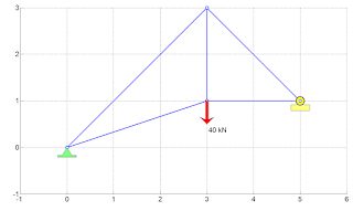
case 10
NODE=[0 0;3 1;5 1;3 3];
ELEM=[1 2;1 4;2 4;2 3;3 4];
drawtruss2D(NODE,ELEM,{{'F',2,90,'40 kN',1},{'R',3,0,' '},{'H',1,0,' '}});
case 11
NODE=[0 0;0.5 -sind(60);1.5 -sind(60);2 0;1.5 sind(60);1 0];
ELEM=[1 2;2 3;3 4;4 5;5 6;1 6;2 6;3 6;4 6;];
drawtruss2D(NODE,ELEM,{{'F',5,0,'100 kN',1},{'R',3,0,' '},{'H',1,90,' '}});
case 12
NODE=[0 0;0 3;0 6;4 0;4 3;4 6];
ELEM=[1 2;2 3;1 4;2 4;2 5;3 5;3 6;4 5;5 6];
drawtruss2D(NODE,ELEM,{{'F',6,0,'100 kN',1},{'R',4,0,' '},{'H',1,0,' '}});

end

Output plots:

Wednesday, 14 November 2018

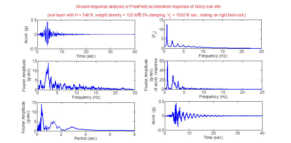
MATLAB program for Ground response analysis or FreeField acceleration response of Gilroy soil site

Ground response analysis or FreeField acceleration response of Gilroy soil site

(soil layer with H = 540 ft, weight density = 125 lb/ft^3, 5% damping, V_s = 1500 ft/ sec, resting on rigid bed-rock)

Ref: Kramer 1996, Example 7.2 in page 262

Fig. 1. Soil layer resting on rigid bed-rock

Gilroy Ground motion (Gilroy# 1, Rock) - Acceleration time history data

https://strongmotioncenter.org/vdc/scripts/stnpage.plx?stations=563

Steps in the MATLAB program for free-field analysis

1. The acceleration time history given in the above table is saved as MATLAB data file Gilroy1_ATH.mat. This is the acceleration at the bed-rock below the soil laer.

2. It is padded with zeros for end-correction in DFT

3. Fft() function is used to split the time history into harmonics

4. Also, the transfer function (F2) is generated for each frequency

5. Product of fft() and transfer function gives the frequency response of acceleration at the top of the soil site

6. To get the time response of acceleration at the top of the soil, ifft() function is used

MATLAB Program

% Importing the ground motion time history

clear;clc;

load ('Gilroy1_ATH.mat');dt=0.02;H=540;ro=125/32.2;G=(ro)*1500^2;zi=0.05;

N=length(data);N=2^(ceil(log2(N)));data=[data;zeros(N-length(data),1)];

t=dt*(1:N)';freq=(1:N)'/dt/N;

figure;subplot(3,2,1);plot(t,data);

FAmp=fft(data);absFAmp=abs(FAmp(1:N/2));

subplot(3,2,3);plot(freq(1:N/2),absFAmp);

subplot(3,2,5);plot(1./freq( 1:N/2),absFAmp);

w=2*pi*freq;vs_=sqrt(G*(1+2*1i*zi)/ro);

F2=1./cos(w*H/vs_);absF2=abs(F2);

subplot(3,2,2);plot(freq(1:N/2),absF2(1:N/2));

Afw=F2.*FAmp;%Afw=abs(F2).*abs(FAmp);%

subplot(3,2,4);plot(freq(1:N/2),abs(Afw(1:N/2)));

Aft=ifft(Afw);

subplot(3,2,6);plot(t,Aft);

Results

Saturday, 30 June 2018

Deflection to BMD

Introduction: In many problems of structural mechanics, the deflection curve of a beam is obtained.
The displacement- based finite element method is one such process that gives deflections/ displacements/
deformations as the first level output, displacement being the field variable. Further quantities of interest
needs to be derived from this basic solution. Here, I present a working procedure using MATLAB code
for generating the BMD and SFD from deflection curve following the assumptions of pure bending under
small deformations.

Algorithm:

Step1: Fit a polynomial of degree ‘n’ for the deflection data

Step2: Obtain the first derivative of the polynomial fit

Step3: Obtain the second derivative of the polynomial fit. This gives curvature

Step4: Multiply the curvature with flexural rigidity ‘EI’ of the beam to get BMD

MATLAB Code:

function [slope,curvature,BMD]=Deflection2BMD(x,y,EI,Order)

f=fittype(['poly' num2str(Order)]);%f = fittype('cubicinterp');

fit1 = fit(x,y,f);

[d1,d2] = differentiate(fit1,x);

subplot(3,2,1);

plot(fit1,x,y);ylabel('Deflection, y');% cfit plot method

subplot(3,2,3);

area(x,d1,'Facecolor','m'); ylabel('Rotation, dy/dx');% double plot method

grid on

legend('1st derivative')

subplot(3,2,5);

area(x,d2,'Facecolor','y');ylabel('Curvature, d^2y/dx^2'); % double plot method

grid on

legend('2nd derivative')

slope=d1;curvature=d2;BMD=d2*EI;

end

Illustration:

Let us consider a cantilever steel beam of cross-sectional dimensions 250 mm x 300 mm (Very heavy ofcourse !!!)
modelled by 3D soild/ brick/ hexhedral elements using Finite Element Analysis, under gravity loading.
The beam is 4 m long. After completing the static stress analysis of the model under self-weight (gravity),
we can easily obtain the deflection curve of the axis of the beam. This is used as the input for the above
MATLAB function. The following is the result of the analysis.

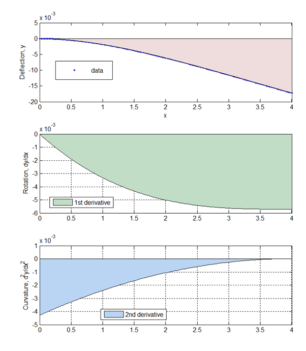
By multiplying the last figure with EI, w get the BMD. It can be seen that the bending moment at the fixed end
is 481 kN-m (taking E=2E11 Pa). This is almost equal to the actual bending moment of a 4 m long cantilever
beam with a UDL of 6000 N/m (which is the self-weight of the beam taking 8000 kg/m3 as the density of steel).