ILD are drawn for a single unit concentrated load travelling on the span/ structure. In the following video, I tried to explain the application of concept of ILD to the analysis of static/moving loads other than unit load, other than concentrated loads, and for multiple loads.
Tuesday, 14 April 2020
ILD for trusses in which panel points are not vertically in line with loaded panel points
In the following video, I tried to explain the procedure for drawing ILDs for member forces in trusses in which the top and bottom panel points are not vertically in line. In such trusses, a small correction needs to be done in the ILD. There should not be an abrupt change in the ILD at the point or section where the loading does not appear directly. So, that abrupt change at non-loading panel points needs to be smoothened.
Saturday, 11 April 2020
ILD s for Simply supported Bridge Trusses
The following video is for the students of II year B. Tech (civil Engineering) Programme. The video details the procedure for drawing ILDs of simply supported trusses
Wednesday, 8 April 2020
Unit Load method for deflections of rigid frames
The following video is for II year under graduate students of Civil Engineering Programme
Strain energy method for slopes and Deflection of beams
The following video is made for students of II year of Bachelor's programme in Civil Engineering
Friday, 15 February 2019
PLotting truss structures using MATLAB code
Objective: The following article explains the MATLAB code to plot a figure of truss structure to scale
MATLAB Functions used: line( ), min( ), max( ), length( ), viscircles( ), patch( ), etc
Other features: THe supports and loading are also depicted in the plots. The load values and directions are clearly indicated in color
MATLAB Code:
function drawtruss2D(NODE,ELEM,L_BC)
figure;line([NODE(ELEM(:,1),1) NODE(ELEM(:,2),1)]',[NODE(ELEM(:,1),2) ...
NODE(ELEM(:,2),2)]','Color','b','LineWidth',2,'Marker','o',...
'MArkerSize',8,'MarkerFacecolor','w');hold on;
minX=min(NODE(:,1));maxX=max(NODE(:,1));minY=min(NODE(:,2));maxY=max(NODE(:,2));
rangeX=maxX-minX;rangeY=maxY-minY;
xlim([minX-0.2*rangeX maxX+0.2*rangeX]);ylim([minY-0.2*rangeY maxY+0.2*rangeY]);
axis equal
if nargin==3
nl=rangeX*0.10;nb=rangeY*0.05;
for o=1:length(L_BC)
OType= L_BC{o}{1};
switch OType
case 'F'
X=[0;-nl*0.30;-nl*0.20;-nl;-nl;-nl*0.20;-nl*0.30;0];
Y=[0;nb;nb*0.2;nb*0.2;-nb*0.2;-nb*0.2;-nb;0]*0.7;
if length(L_BC{o})>4;X=X+nl;end
F=L_BC{o}{2};rot=L_BC{o}{3};
theta=rot/180*pi;
R = [cos(theta) -sin(theta); sin(theta) cos(theta)];
Trans=[X Y]*R;Xt=Trans(:,1);Yt=Trans(:,2);
Xf=NODE(F,1);Yf=NODE(F,2);
patch(Xt+Xf,Yt+Yf,[1 0 0]);
Xa=[nl*0.25 nb*0.25]*R;
if length(L_BC{o})>4;text(Xt(1)+Xf+Xa(1),Yt(1)+Yf+Xa(2),L_BC{o}{4},'FontSize',18);
else text(Xt(4)+Xf+Xa(1),Yt(4)+Yf+Xa(2),L_BC{o}{4},'FontSize',18);end
case 'H'
X=[0;-nl/4;-nl/2;-nl/2;nl/2;nl/2;nl/4;0];
Y=[0;-nb*0.8;-nb*0.8;-nb;-nb;-nb*0.8;-nb*0.8;0]*1.2;
F=L_BC{o}{2};rot=L_BC{o}{3};
theta=rot/180*pi;
R = [cos(theta) -sin(theta); sin(theta) cos(theta)];
Trans=[X Y]*R;Xt=Trans(:,1);Yt=Trans(:,2);
Xf=NODE(F,1);Yf=NODE(F,2);
patch(Xt+Xf,Yt+Yf,[0.5 1 0.5]);
case 'R'
X=[-nl/2;-nl/2;nl/2;nl/2];
Y=[-nb*0.4;-nb;-nb;-nb*0.4]*1.2;
F=L_BC{o}{2};rot=L_BC{o}{3};
theta=rot/180*pi;
R = [cos(theta) -sin(theta); sin(theta) cos(theta)];
Trans=[X Y]*R;Xt=Trans(:,1);Yt=Trans(:,2);
Xf=NODE(F,1);Yf=NODE(F,2);
patch(Xt+Xf,Yt+Yf,[1 1 0.5]);
viscircles([0 0]*R+[Xf Yf],nb*0.4,'LineWidth',5,'EdgeColor','y');
viscircles([0 0]*R+[Xf Yf],nb*0.6,'EdgeColor','k');
end
end
end
return
Typical input Files:
%Truss data for various problems
FlagNo=12;
switch FlagNo
case 1 % Single Braced Truss %Page 693 Vazirani and Ratwani
NODET=[0 0;8 0];NODE=[];for i=1:5;NODE=[NODE;NODET+[[0;0] 6*[i-1;i-1]]];end
ELEMT=[1 3;1 4; 3 4 ;2 4];ELEM=[];for i=1:4;ELEM=[ELEM;ELEMT+(i-1)*2];end
drawtruss2D(NODE,ELEM,{{'F',3,0,'30 kN',1},{'F',4,180,'30 kN'},{'R',2,0,'30 kN'},{'H',1,0,'30 kN'}});
case 2 %
NODET=[3 0;3 4;6 0;6 8];NODE=[0 0;0 8];n=4;
for i=1:n
NODE=[NODE;NODET+[6*(i-1)*ones(4,1) zeros(4,1)]];
end
ELEMT=[1 3;1 4; 2 4;3 5;4 5;2 6;5 6];ELEM=[1 2];
ELEMT1=[1 3;1 4; 3 5;4 5;4 6;2 6;5 6];
for i=1:n
if i<=n/2
ELEM=[ELEM;ELEMT+4*(i-1)];
else
ELEM=[ELEM;ELEMT1+4*(i-1)];
end
end
drawtruss2D(NODE,ELEM);
case 3 %Page 11 Vazirani
NODE=[0 0;0 4;4 2;4 6;8 4;8 8;12 4;12 8;16 0;16 4;20 -4;20 0];
ELEM=[1 2;1 3;2 3;2 4;3 4; 3 5; 4 5; 4 6; 5 6;5 7;6 8;7 8;7 9;7 10;8 10;9 10;9 11;9 12;10 12;11 12];
drawtruss2D(NODE,ELEM,{{'F',4,90,'30 kN'},{'H',1,0,'30 kN'},{'H',11,0,'30 kN'}});
case 4 %PAge 51, Negi and Jangid
NODE=[0 0;4 0; 8 0;8 -4;4 -2];
ELEM=[1 2;1 5;2 5;2 3;5 3; 5 4;3 4];
drawtruss2D(NODE,ELEM,{{'F',1,90,'P'},{'F',2,90,'P'},{'F',3,90,'P'},{'R',1,30,' '},{'H',4,0,' '}});
case 5 %PAge 51b, Negi and Jangid
NODE=[0 0;3 3; 3 0;6 6;6 0;9 9;9 0;12 6;12 0;15 3;15 0;18 0];
ELEM=[1 2;1 3;2 3;2 4;2 5; 3 5;5 4;4 6;4 7;5 7;7 6;6 8;7 8;7 9;9 8;8 10;9 10;9 11;11 10;10 12;11 12];
drawtruss2D(NODE,ELEM,{{'F',7,90,'P',1},{'R',12,0,' '},{'H',1,0,' '}});
case 6
NODE=[0 0;3 3*sqrt(3); 6 0;2.25 2.25;3.75 2.25;3 3*tand(15)];
ELEM=[1 2;2 3;3 1;1 4;2 5;3 6;4 5;5 6;6 4];
drawtruss2D(NODE,ELEM,{{'F',6,90,'P',1},{'R',3,0,' '},{'H',1,0,' '}});
case 7
NODE=[0 0;3 0;6 3;6 6;3 3;0 3];
ELEM=[1 2;2 3;3 4;4 5;5 6;6 1;1 5;5 2;5 3];
drawtruss2D(NODE,ELEM,{{'F',4,0,'H',1},{'F',4,270,'W',1},{'R',6,90,' '},{'H',1,90,' '}});
case 8
NODE=[0 0;8 0;4 3;4 0];
ELEM=[1 3;1 4;3 4;3 2;4 2];
drawtruss2D(NODE,ELEM,{{'F',4,90,'15 kN',1},{'R',2,0,' '},{'H',1,0,' '}});
case 9
NODE=[0 0;0 4;4 4;4 0];
ELEM=[1 2;1 3;1 4;2 3;3 4];
drawtruss2D(NODE,ELEM,{{'F',2,0,'P'},{'R',4,0,' '},{'H',1,0,' '}});
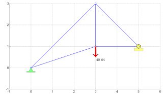
case 10
NODE=[0 0;3 1;5 1;3 3];
ELEM=[1 2;1 4;2 4;2 3;3 4];
drawtruss2D(NODE,ELEM,{{'F',2,90,'40 kN',1},{'R',3,0,' '},{'H',1,0,' '}});
case 11
NODE=[0 0;0.5 -sind(60);1.5 -sind(60);2 0;1.5 sind(60);1 0];
ELEM=[1 2;2 3;3 4;4 5;5 6;1 6;2 6;3 6;4 6;];
drawtruss2D(NODE,ELEM,{{'F',5,0,'100 kN',1},{'R',3,0,' '},{'H',1,90,' '}});
case 12
NODE=[0 0;0 3;0 6;4 0;4 3;4 6];
ELEM=[1 2;2 3;1 4;2 4;2 5;3 5;3 6;4 5;5 6];
drawtruss2D(NODE,ELEM,{{'F',6,0,'100 kN',1},{'R',4,0,' '},{'H',1,0,' '}});
end
Output plots:


MATLAB Functions used: line( ), min( ), max( ), length( ), viscircles( ), patch( ), etc
Other features: THe supports and loading are also depicted in the plots. The load values and directions are clearly indicated in color
MATLAB Code:
function drawtruss2D(NODE,ELEM,L_BC)
figure;line([NODE(ELEM(:,1),1) NODE(ELEM(:,2),1)]',[NODE(ELEM(:,1),2) ...
NODE(ELEM(:,2),2)]','Color','b','LineWidth',2,'Marker','o',...
'MArkerSize',8,'MarkerFacecolor','w');hold on;
minX=min(NODE(:,1));maxX=max(NODE(:,1));minY=min(NODE(:,2));maxY=max(NODE(:,2));
rangeX=maxX-minX;rangeY=maxY-minY;
xlim([minX-0.2*rangeX maxX+0.2*rangeX]);ylim([minY-0.2*rangeY maxY+0.2*rangeY]);
axis equal
if nargin==3
nl=rangeX*0.10;nb=rangeY*0.05;
for o=1:length(L_BC)
OType= L_BC{o}{1};
switch OType
case 'F'
X=[0;-nl*0.30;-nl*0.20;-nl;-nl;-nl*0.20;-nl*0.30;0];
Y=[0;nb;nb*0.2;nb*0.2;-nb*0.2;-nb*0.2;-nb;0]*0.7;
if length(L_BC{o})>4;X=X+nl;end
F=L_BC{o}{2};rot=L_BC{o}{3};
theta=rot/180*pi;
R = [cos(theta) -sin(theta); sin(theta) cos(theta)];
Trans=[X Y]*R;Xt=Trans(:,1);Yt=Trans(:,2);
Xf=NODE(F,1);Yf=NODE(F,2);
patch(Xt+Xf,Yt+Yf,[1 0 0]);
Xa=[nl*0.25 nb*0.25]*R;
if length(L_BC{o})>4;text(Xt(1)+Xf+Xa(1),Yt(1)+Yf+Xa(2),L_BC{o}{4},'FontSize',18);
else text(Xt(4)+Xf+Xa(1),Yt(4)+Yf+Xa(2),L_BC{o}{4},'FontSize',18);end
case 'H'
X=[0;-nl/4;-nl/2;-nl/2;nl/2;nl/2;nl/4;0];
Y=[0;-nb*0.8;-nb*0.8;-nb;-nb;-nb*0.8;-nb*0.8;0]*1.2;
F=L_BC{o}{2};rot=L_BC{o}{3};
theta=rot/180*pi;
R = [cos(theta) -sin(theta); sin(theta) cos(theta)];
Trans=[X Y]*R;Xt=Trans(:,1);Yt=Trans(:,2);
Xf=NODE(F,1);Yf=NODE(F,2);
patch(Xt+Xf,Yt+Yf,[0.5 1 0.5]);
case 'R'
X=[-nl/2;-nl/2;nl/2;nl/2];
Y=[-nb*0.4;-nb;-nb;-nb*0.4]*1.2;
F=L_BC{o}{2};rot=L_BC{o}{3};
theta=rot/180*pi;
R = [cos(theta) -sin(theta); sin(theta) cos(theta)];
Trans=[X Y]*R;Xt=Trans(:,1);Yt=Trans(:,2);
Xf=NODE(F,1);Yf=NODE(F,2);
patch(Xt+Xf,Yt+Yf,[1 1 0.5]);
viscircles([0 0]*R+[Xf Yf],nb*0.4,'LineWidth',5,'EdgeColor','y');
viscircles([0 0]*R+[Xf Yf],nb*0.6,'EdgeColor','k');
end
end
end
return
Typical input Files:
%Truss data for various problems
FlagNo=12;
switch FlagNo
case 1 % Single Braced Truss %Page 693 Vazirani and Ratwani
NODET=[0 0;8 0];NODE=[];for i=1:5;NODE=[NODE;NODET+[[0;0] 6*[i-1;i-1]]];end
ELEMT=[1 3;1 4; 3 4 ;2 4];ELEM=[];for i=1:4;ELEM=[ELEM;ELEMT+(i-1)*2];end
drawtruss2D(NODE,ELEM,{{'F',3,0,'30 kN',1},{'F',4,180,'30 kN'},{'R',2,0,'30 kN'},{'H',1,0,'30 kN'}});
case 2 %
NODET=[3 0;3 4;6 0;6 8];NODE=[0 0;0 8];n=4;
for i=1:n
NODE=[NODE;NODET+[6*(i-1)*ones(4,1) zeros(4,1)]];
end
ELEMT=[1 3;1 4; 2 4;3 5;4 5;2 6;5 6];ELEM=[1 2];
ELEMT1=[1 3;1 4; 3 5;4 5;4 6;2 6;5 6];
for i=1:n
if i<=n/2
ELEM=[ELEM;ELEMT+4*(i-1)];
else
ELEM=[ELEM;ELEMT1+4*(i-1)];
end
end
drawtruss2D(NODE,ELEM);
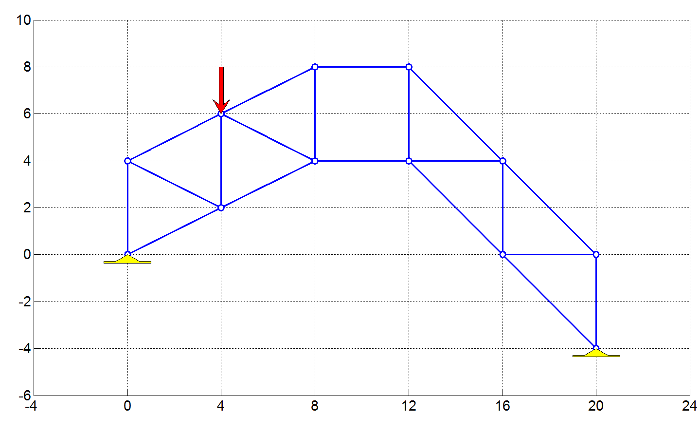
case 3 %Page 11 Vazirani
NODE=[0 0;0 4;4 2;4 6;8 4;8 8;12 4;12 8;16 0;16 4;20 -4;20 0];
ELEM=[1 2;1 3;2 3;2 4;3 4; 3 5; 4 5; 4 6; 5 6;5 7;6 8;7 8;7 9;7 10;8 10;9 10;9 11;9 12;10 12;11 12];
drawtruss2D(NODE,ELEM,{{'F',4,90,'30 kN'},{'H',1,0,'30 kN'},{'H',11,0,'30 kN'}});
case 4 %PAge 51, Negi and Jangid
NODE=[0 0;4 0; 8 0;8 -4;4 -2];
ELEM=[1 2;1 5;2 5;2 3;5 3; 5 4;3 4];
drawtruss2D(NODE,ELEM,{{'F',1,90,'P'},{'F',2,90,'P'},{'F',3,90,'P'},{'R',1,30,' '},{'H',4,0,' '}});
case 5 %PAge 51b, Negi and Jangid
NODE=[0 0;3 3; 3 0;6 6;6 0;9 9;9 0;12 6;12 0;15 3;15 0;18 0];
ELEM=[1 2;1 3;2 3;2 4;2 5; 3 5;5 4;4 6;4 7;5 7;7 6;6 8;7 8;7 9;9 8;8 10;9 10;9 11;11 10;10 12;11 12];
drawtruss2D(NODE,ELEM,{{'F',7,90,'P',1},{'R',12,0,' '},{'H',1,0,' '}});
case 6
NODE=[0 0;3 3*sqrt(3); 6 0;2.25 2.25;3.75 2.25;3 3*tand(15)];
ELEM=[1 2;2 3;3 1;1 4;2 5;3 6;4 5;5 6;6 4];
drawtruss2D(NODE,ELEM,{{'F',6,90,'P',1},{'R',3,0,' '},{'H',1,0,' '}});
case 7
NODE=[0 0;3 0;6 3;6 6;3 3;0 3];
ELEM=[1 2;2 3;3 4;4 5;5 6;6 1;1 5;5 2;5 3];
drawtruss2D(NODE,ELEM,{{'F',4,0,'H',1},{'F',4,270,'W',1},{'R',6,90,' '},{'H',1,90,' '}});
case 8
NODE=[0 0;8 0;4 3;4 0];
ELEM=[1 3;1 4;3 4;3 2;4 2];
drawtruss2D(NODE,ELEM,{{'F',4,90,'15 kN',1},{'R',2,0,' '},{'H',1,0,' '}});
case 9
NODE=[0 0;0 4;4 4;4 0];
ELEM=[1 2;1 3;1 4;2 3;3 4];
drawtruss2D(NODE,ELEM,{{'F',2,0,'P'},{'R',4,0,' '},{'H',1,0,' '}});
case 10
NODE=[0 0;3 1;5 1;3 3];
ELEM=[1 2;1 4;2 4;2 3;3 4];
drawtruss2D(NODE,ELEM,{{'F',2,90,'40 kN',1},{'R',3,0,' '},{'H',1,0,' '}});
case 11
NODE=[0 0;0.5 -sind(60);1.5 -sind(60);2 0;1.5 sind(60);1 0];
ELEM=[1 2;2 3;3 4;4 5;5 6;1 6;2 6;3 6;4 6;];
drawtruss2D(NODE,ELEM,{{'F',5,0,'100 kN',1},{'R',3,0,' '},{'H',1,90,' '}});
case 12
NODE=[0 0;0 3;0 6;4 0;4 3;4 6];
ELEM=[1 2;2 3;1 4;2 4;2 5;3 5;3 6;4 5;5 6];
drawtruss2D(NODE,ELEM,{{'F',6,0,'100 kN',1},{'R',4,0,' '},{'H',1,0,' '}});
end
Output plots:


Wednesday, 14 November 2018
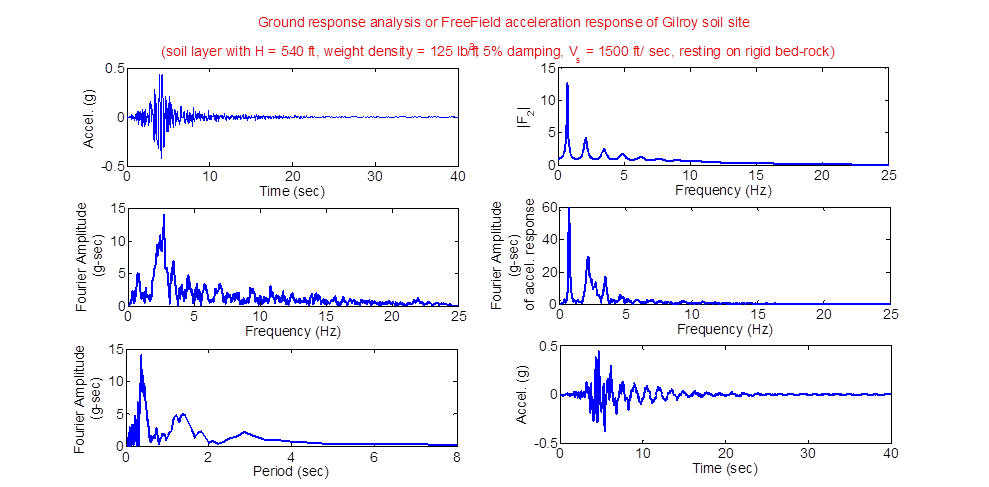
MATLAB program for Ground response analysis or FreeField acceleration response of Gilroy soil site
Ground response analysis or FreeField acceleration response of Gilroy soil site
(soil layer with H = 540 ft, weight density = 125 lb/ft^3, 5% damping, V_s = 1500 ft/ sec, resting on rigid bed-rock)
Ref: Kramer 1996, Example 7.2 in page 262

Fig. 1. Soil layer resting on rigid bed-rock
Gilroy Ground motion (Gilroy# 1, Rock) - Acceleration time history data
Steps in the MATLAB program for free-field analysis
1. The acceleration time history given in the above table is saved as MATLAB data file Gilroy1_ATH.mat. This is the acceleration at the bed-rock below the soil laer.
2. It is padded with zeros for end-correction in DFT
3. Fft() function is used to split the time history into harmonics
4. Also, the transfer function (F2) is generated for each frequency
5. Product of fft() and transfer function gives the frequency response of acceleration at the top of the soil site
6. To get the time response of acceleration at the top of the soil, ifft() function is used
MATLAB Program
% Importing the ground motion time history
clear;clc;
load ('Gilroy1_ATH.mat');dt=0.02;H=540;ro=125/32.2;G=(ro)*1500^2;zi=0.05;
N=length(data);N=2^(ceil(log2(N)));data=[data;zeros(N-length(data),1)];
t=dt*(1:N)';freq=(1:N)'/dt/N;
figure;subplot(3,2,1);plot(t,data);
FAmp=fft(data);absFAmp=abs(FAmp(1:N/2));
subplot(3,2,3);plot(freq(1:N/2),absFAmp);
subplot(3,2,5);plot(1./freq( 1:N/2),absFAmp);
w=2*pi*freq;vs_=sqrt(G*(1+2*1i*zi)/ro);
F2=1./cos(w*H/vs_);absF2=abs(F2);
subplot(3,2,2);plot(freq(1:N/2),absF2(1:N/2));
Afw=F2.*FAmp;%Afw=abs(F2).*abs(FAmp);%
subplot(3,2,4);plot(freq(1:N/2),abs(Afw(1:N/2)));
Aft=ifft(Afw);
subplot(3,2,6);plot(t,Aft);
|
Results
Subscribe to:
Posts (Atom)